2024-04-15发表2026-02-14更新实用技术18 分钟读完 (大约2652个字)

SPEI计算的原理与算法优化

什么是SPEI

标准化降水蒸散指数SPEI（Standardized Precipitation Evapotranspiration Index）可以表征干湿状态。
SPEI值越大越湿润，越小越干旱，其最早由Sergio M. Vicente-Serrano等人提出。

SPEI算法

注意：这里的SPEI计算方法存在一些缺陷。目前已经基于其他包并行化之后的算法对其进行修改，请等待博客后续更新。

构建差值序列

首先构建降水量$P_i$和潜在蒸散发$PET_i$的差值序列$D_i$，

$$ D_i = P_i-PET_i $$

可以选定不同的时间尺度来计算SPEI。时间尺度为$k$，$i$日的$D_i$累计为该日前$k$天的$D_i$之和，也就是说，对于每个$k$尺度的$D_i$，其为前$k$天的滑动窗口和。

对差值序列进行拟合

目前常见的SPEI拟合方法均为使用三参数Log-Logistic分布（也称Fisk分布）对$D_i$进行拟合。近几年的研究显示，Genextreme分布对SPEI有更好的拟合效果。

Python在GIS系统中有其重要的生态位，但是使用Python对SPEI进行计算十分低效。传统方法中，若使用Scipy和循环进行Fisk分布的参数估计，计算大型数据集将十分困难，考虑如下代码：

import numpy as np

def calc_spei_fisk_paras(d_i_matrix:np.ndarray) -> np.ndarray:
    from scipy.stats import fisk

    d_i_shape = d_i_matrix.shape # d_i_matrix is the numpy array with the shape (time,x,y)

    paras = np.zeros_like(d_i_shape)[0:3,:,:] # Storage fisk distribution paras

    for i in d_i_shape[1]:
        for j in d_i_shape[2]:
            paras[:,i,j] = fisk.fit(d_i_matrix[:,i,j])

    return paras

该函数使用二重嵌套循环对SPEI进行计算，因为Python的特性，该段代码的执行将极度缓慢，面对高分辨率图象时尤其明显。要对该算法进行优化，有以下几个方向：

循环向量化
寻找新的参数估计模式
jit编译

概率值正态化

序列值代入已估计参数的Genextreme分布得到概率值$P_i$；之后将概率值代入标准正态分布累积分布函数的反函数，得到SPEI值：

$$ \mathrm{SPEI}_i = \Phi^{-1}(P_i) $$

算法优化

循环向量化

循环向量化指将使用循环进行的操作改为操作向量，C语言在编译时编译器会自动地将循环优化成处理器支持的SIMD指令。

SIMD(Single Instruction Multiple Data)即单指令流多数据流，是一种采用一个控制器来控制多个处理器，同时对一组数据（又称“数据向量”）中的每一个分别执行相同的操作从而实现空间上的并行性的技术。

考虑以下C代码，

/*
simd.c
Test the simd optimization support for gcc
 */
#include <stdio.h>
#define LENGTH(array) (sizeof(array) / sizeof(array[0]))

int main() {
    int vec1[3];
    int vec2[3];
    printf("Input the First Vec:\n");
    scanf("%d%d%d", &vec1[0], &vec1[1], &vec1[2]);
    printf("Input the Secound Vec:\n");
    scanf("%d%d%d", &vec2[0], &vec2[1], &vec2[2]);

    int vec3[3];

    for (int i = 0; i < LENGTH(vec1); i++) {
        vec3[i] = vec1[i] + vec2[i];
    }

    printf("Sum Vector is %d %d %d\n", vec3[0], vec3[1], vec3[2]);

    return 0;
}

该程序将两个int类型的变量使用循环相加。在AMD64机器上使用gcc的-O1和-O3优化选项分别编译得到汇编文件（也可以去网站Compiler Explorer）：

1
2
3

gcc simd.c -S -o simd_O1.S -masm=intel -march=core-avx2 -O1 -v

gcc simd.c -S -o simd_O3.S -masm=intel -march=core-avx2 -O3 -v

汇编文件分别为：

# simd_O1.S
.LC0:
        .string "Input the First Vec:"
.LC1:
        .string "%d%d%d"
.LC2:
        .string "Input the Secound Vec:"
.LC3:
        .string "Sum Vector is %d %d %d\n"
main:
        sub     rsp, 40
        mov     edi, OFFSET FLAT:.LC0
        call    puts
        lea     rsi, [rsp+20]
        lea     rcx, [rsp+28]
        lea     rdx, [rsp+24]
        mov     edi, OFFSET FLAT:.LC1
        mov     eax, 0
        call    __isoc99_scanf
        mov     edi, OFFSET FLAT:.LC2
        call    puts
        lea     rsi, [rsp+8]
        lea     rcx, [rsp+16]
        lea     rdx, [rsp+12]
        mov     edi, OFFSET FLAT:.LC1
        mov     eax, 0
        call    __isoc99_scanf
        mov     ecx, DWORD PTR [rsp+16]
        add     ecx, DWORD PTR [rsp+28]
        mov     edx, DWORD PTR [rsp+12]
        add     edx, DWORD PTR [rsp+24]
        mov     esi, DWORD PTR [rsp+8]
        add     esi, DWORD PTR [rsp+20]
        mov     edi, OFFSET FLAT:.LC3
        mov     eax, 0
        call    printf
        mov     eax, 0
        add     rsp, 40
        ret

# simd_O3.S
.LC0:
        .string "Input the First Vec:"
.LC1:
        .string "%d%d%d"
.LC2:
        .string "Input the Secound Vec:"
.LC3:
        .string "Sum Vector is %d %d %d\n"
main:
        push    rbp
        mov     edi, OFFSET FLAT:.LC0
        mov     rbp, rsp
        and     rsp, -32
        sub     rsp, 64
        call    puts
        mov     rsi, rsp
        lea     rcx, [rsp+8]
        xor     eax, eax
        lea     rdx, [rsp+4]
        mov     edi, OFFSET FLAT:.LC1
        call    __isoc99_scanf
        mov     edi, OFFSET FLAT:.LC2
        call    puts
        lea     rsi, [rsp+32]
        lea     rcx, [rsp+40]
        xor     eax, eax
        lea     rdx, [rsp+36]
        mov     edi, OFFSET FLAT:.LC1
        call    __isoc99_scanf
        vmovq   xmm0, QWORD PTR [rsp]
        mov     ecx, DWORD PTR [rsp+40]
        xor     eax, eax
        vmovq   xmm1, QWORD PTR [rsp+32]
        add     ecx, DWORD PTR [rsp+8]
        mov     edi, OFFSET FLAT:.LC3
        vpaddd  xmm0, xmm0, xmm1
        vpextrd edx, xmm0, 1
        vmovd   esi, xmm0
        call    printf
        xor     eax, eax
        leave
        ret

在没有使用优化的情况下，程序使用了3条addl指令，而优化过后其使用了xmm寄存器（SSE指令集）提升了计算效率。但Python解释器没有内建的SIMD支持，要解决这种问题可以使用numpy包：

import numpy as np
import timeit

def sum_numpy(a:np.ndarray, b:np.ndarray) -> np.ndarray:
    return np.sum(a + b)


def sum_circulate(a:np.ndarray, b:np.ndarray) -> np.ndarray:
    n = len(a)
    c = np.zeros(n)
    for i in range(n):
        c[i] = a[i] + b[i]
    return np.sum(c)


a = np.random.rand(10000)
b = np.random.rand(10000)

print(timeit.timeit(lambda: sum_numpy(a, b), number=100))
print(timeit.timeit(lambda: sum_circulate(a, b), number=100))

输出结果不难预测，

1 2	0.004135900000619586 0.6949793999992835

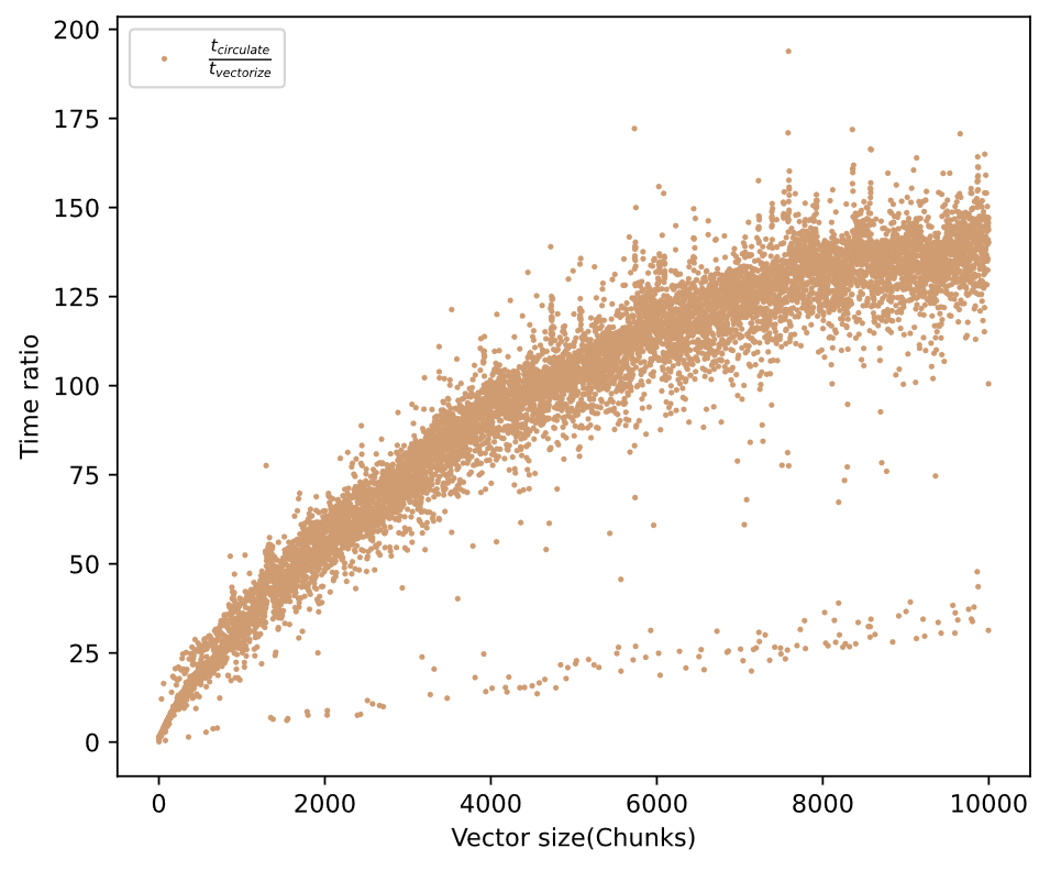
numpy版本的向量加法比循环版本快了170多倍。如果我们以数组规模和所用时间作图，我们得到以下结果：

时间比较

问题规模越大，SIMD带来的加速效果越明显。但是scipy中的参数估计方法无法实现循环向量化，一次只能处理一个时间序列；而且修改scipy中的代码的成本又太高（大部分代码均由C语言写成），所以需要找新的参数估计模式。

Genextreme分布与L-moments

Genextreme分布是相对更好的SPEI拟合的候选分布。其参数估计可以简单的使用L-moments估计得到。

使用L-moments的参数估计过程可以由以下公式给出：

GEV分布的CDF为

\begin{equation}
F(x)=\left\{
\begin{aligned}
\mathrm{exp}(-(1-\kappa\frac{x-\xi}{\alpha})^{1/\kappa}),\kappa\not= 0 \\
\mathrm{exp}(\mathrm{exp}(-\frac{x-\xi}{\alpha})),\kappa = 0
\end{aligned}
\right.
\end{equation}

其中$\alpha,\xi,\kappa$为参数。

记L-mean，L-scale，L-skewness分别为$\lambda_1,\lambda_2,\tau_3$，GEV分布的三个参数可以用如下公式近似估计：

\begin{equation}
\kappa =\left\{
\begin{aligned}
&0.488138(\tau_3)^{1.70839}-1.7631(\tau_3)^{0.981824}+0.285706, 0.01\le\tau_3\le 0.5 \\
&0.483706(\tau_3)^{1.679096}-1.73786(\tau_3)^{1.008948}+0.255108, 0.5\le\tau_3\le 0.95
\end{aligned}
\right.
\end{equation}

\begin{equation}
\frac{\alpha}{\lambda_2}=\left\{
\begin{aligned}
&1.023602813(\tau_3)^{1.8850974}-2.95087636(\tau_3)^{1.195591244}+1.7599614982, -0.5\le \kappa \le 0.3 \\
&1.5954866(\tau_3)^{1.5816175}-3.886135(\tau_3)^{0.89522}+2.310643, \kappa > 0.3
\end{aligned}
\right.
\end{equation}

\begin{equation}
\frac{\xi-\lambda_1}{\lambda_2}=-0.0937(\tau_3)^4-0.2198(\tau_3)^3+1.407(\tau_3)^2-1.4825(\tau_3)-0.6205, 0.01\le\tau_3\le 0.95
\end{equation}

线性矩$\lambda_1,\lambda_2,\tau_3$可以使用lmoments3包中的代码修改而来。lmoments3包中的线性矩计算方法可以简单的进行修改，以实现循环向量化：

# Here are just a few of the key codes
import numpy as np
import numba as nb # numba jit, which will be introduced next
...
@nb.njit(nb.float64[:, :, :](nb.float64[:, :, :], nb.int8), parallel=True, cache=True)
def get_lratios_jit(x: np.ndarray, nmom: int = 5) -> np.ndarray:
    """
    Calculates L-moments (up to the specified order) of an array of data using Numba JIT compilation.

    Args:
        x (np.ndarray): A 3D array of data.
        nmom (int, optional): The order of L-moments to compute (default is 5).

    Returns:
        np.ndarray: An array containing L-moments up to the specified order.
    """
    def sort_array_with_axis(x: np.ndarray, axis: int) -> np.ndarray:
        """
        Sorts the input array along the specified axis.

        Args:
            x (np.ndarray): Input array.
            axis (int): Axis along which to sort.

        Returns:
            np.ndarray: Sorted array.
        """
        for i in nb.prange(x.shape[axis]):
            x[i] = np.sort(x[i])
        return x

    x = np.asarray(x, dtype=np.float64)
    n = x.shape[0]

    x = sort_array_with_axis(x, 0)

    sum_xtrans = np.empty_like(x[0])

    def comb(n, r):
        """
        Computes the binomial coefficient (n choose r).

        Args:
            n (int): Total number of items.
            r (int): Number of items to choose.

        Returns:
            int: Binomial coefficient.
        """
        if r < 0 or r > n:
            return 0
        if r == 0 or r == n:
            return 1
        c = 1
        for i in range(1, r + 1):
            c = c * (n - i + 1) // i
        return c

    # First L-moment

    l1 = np.sum(x, axis=0) / comb(n, 1)

    if nmom == 1:
        return np.expand_dims(l1, axis=0)

    # Second L-moment

    comb1 = np.arange(n)
    coefl2 = 0.5 / comb(n, 2)
    sum_xtrans[:] = 0
    for i in nb.prange(n):
        sum_xtrans += (comb1[i] - comb1[n - 1 - i]) * x[i]
    l2 = coefl2 * sum_xtrans

    if nmom == 2:
        return np.stack((l1, l2))

    # Third L-moment

    comb3 = np.zeros(n)
    for i in range(n):
        comb3[i] = comb(i, 2)
    coefl3 = 1.0 / 3.0 / comb(n, 3)
    sum_xtrans[:] = 0
    for i in nb.prange(n):
        sum_xtrans += (
            comb3[i] - 2 * comb1[i] * comb1[n - 1 - i] + comb3[n - 1 - i]
        ) * x[i]
    l3 = coefl3 * sum_xtrans / l2

    if nmom == 3:
        return np.stack((l1, l2, l3))
...

由以上示例代码能计算出$\lambda_1,\lambda_2,\tau_3$，便可以由参数估计的公式给出参数值，进而描述Genextreme分布

jit编译

jit 的全称是 Just-in-time，在我们使用的numba库里面则特指Just-in-time Compilation（即时编译）。因为Python的动态类型带来的低效率，需要使用jit技术加速python代码的运行。在代码第一次被执行时将被编译为高效的机器码，同时也能由编译器执行相应的编译优化，以提高执行效率。但是，numba并不是对所有的Python代码都有优化效果，使用前需要去numba的官方文档查看他支持的python功能和numpy功能。

在上一节中给出的代码就包含了numba包，

import numpy as np
import numba as nb # <- numba jit
...
@nb.njit(nb.float64[:, :, :](nb.float64[:, :, :], nb.int8), parallel=True, cache=True) # <- decorator
def get_lratios_jit(x: np.ndarray, nmom: int = 5) -> np.ndarray:
    ...

注意到使用了@njit函数装饰器，装饰器的参数里给出了输入输出数组的数据类型，以及parallel=True，cache=True等几个选项。他们的意义分别是开启自动循环并行化和编译缓存。这里将仅解释循环并行化，也可以看官方对循环自动并行化的解释。

循环并行化

假设代码在一个多CPU系统上运行，对于类似下文给出的没有交叉迭代以来关系的循环，

@njit(parallel=True)
def test(x):
    n = x.shape[0]
    a = np.sin(x)
    b = np.cos(a * a)
    acc = 0
    for i in prange(n - 2):
        for j in prange(n - 1):
            acc += b[i] + b[j + 1]
    return acc

numba会自动将循环分配到CPU的多个核心上以增加并行度。

后记

文中的完整代码已放于Github仓库pylm-spei。要在正态化的步骤执行加速，可以参考numba-stats。

SPEI计算的原理与算法优化

https://blog.zyzh20021020.cn/posts/3b041e4b/

作者

zyzh0

发布于

2024-04-15

更新于

2026-02-14

许可协议

#SPEI 并行计算

SPEI计算的原理与算法优化

什么是SPEI

SPEI算法

构建差值序列

对差值序列进行拟合

概率值正态化

算法优化

循环向量化

Genextreme分布与L-moments

jit编译

循环并行化

后记

作者

发布于

更新于

许可协议

目录

链接

分类

最新文章

归档

标签

Your browser is out-of-date!